Marginal Propensity to Consume and the Velocity of Money

My last post pointed out my frustration with the treatment of the marginal propensity to consume and the spending multiplier in a traditional principles text.  I just want to briefly point out how this whole business fits nicely into my alternate paradigm where the aggregate demand curve is thought of as PY=MV (as opposed to Y=C+I+G+NX).

Here is how Mateer and Coppock approach the MPC (emphasis added):

When a person’s income rises, he or she might save some of this new income but might be just as likely to spend part of it too.  The marginal propensity to consume (MPC) is the portion of additional income that is spent on consumption.

The problem here is the dichotomy between consumption and saving.  As I have mentioned before, it matters what we mean exactly by “saving.”  Normally (outside of the Keynesian AS/AD model) we assume that saving means investment and investment is also in the CIG equation (it’s the I).  So if “saving” means that you lend part of your income to a firm who buys investment goods, then doesn’t that part of your income become the income of the producer of those investment goods and isn’t that exactly the same as the portion you spent on consumption goods?  (Yes.)  So then is this all just nonsense or is there some grain of truth in here that we are just saying in an idiotic way?

Well, there is one and only one way of saving that is not exactly the same as consuming in the sense that when you do it, the money you devote to it becomes another person’s income.  That way is holding money.  So what happens if we change the way we explain this slightly so that instead of saying that people consume a fraction of their income c and “save” the rest, we say that people spend a fraction of their income c and hold the rest as money and this spending may be on either consumption or investment goods.

Now you can ask yourself “what is the effect on total spending of a given increase in government expenditure.  Let’s assume that the government borrows $100 from the central bank and spends it on something and let’s assume that the marginal propensity to spend (MPS) is 0.9.  Then the person who gets that initial $100 will spend 90 and the person who gets that will spend 81 and so on.  Take that series out to infinity and you will get the total increase in spending of 100/(1-MPS) or the familiar spending multiplier.

But now notice that another way to see this is to notice that people are holding 10% of their income as money and we have increased the money supply by $100.  This means that total incomes (which must equal total spending) must rise by–you guessed it–1/(1-.9) times the change in the money supply.  Or, to put it another way, incomes have to rise enough that people become willing to hold the new money.

But now you are coming strikingly close to another similar concept.  If people are willing to hold 10% of their income as money, that means each dollar in the economy will have to change hands 10 times on average for people to become willing to hold all the money.  Or in other words, the velocity of money will be one over the average propensity to hold money.  (There is, of course, the possibility that the average and marginal propensities may not be the same but that’s not of particular importance to my point.)  And that is just 1-MPS.  So in other words, if you characterize this thing correctly (it’s about spending and not consuming) then the Keynesian spending multiplier just becomes the velocity of money.

Of course, if you look at it this way, you are forced to notice that the real cause of the increase in aggregate demand in this case is an increase in the money supply not something magical about government spending.  If they just dumped the money into the economy from helicopters, the effect would mostly be the same.  And that’s exactly why this way is better, and probably also why it isn’t what we do.

However, there is one magical thing about government spending which is that the government can choose a higher MPS (usually 1) and so can get more spending bang  per dollar of increase in M in the first round.  So the “helicopter multiple” (if you will) would be slightly less ((1/(1-MPS))-1).  And because of this, it becomes theoretically possible that the government could boost aggregate demand without increasing the money supply by borrowing or taxing.

If they increase taxes by $100, they reduce private consumption and/or investment by $100 times the helicopter multiple but then when they spend it they increase private consumption and/or investment by the same amount but with the government spending added on top (assuming that the propensity to spend is unaltered).  This, of course, is a standard fiscal policy implication (see textbook claim 2 in the previous post).  But if you think about it in the context of the equation of exchange, you can actually see what’s going on here.  Essentially, the government is just increasing the velocity of money by taking it away from people and spending it at a higher rate than they would have.

And there you find the special power of government to boost aggregate demand.  Just like the special power of government to do anything else, it boils down to their ability to force people to do a thing more or less.  In this case it’s the ability to force them to spend more money.  The same thing would happen if you put a horde of killer robots on the streets programmed to shoot missiles at anyone they ran across holding any money.  Or, for that matter if–in some crazy, hypothetical, sci-fi universe–all money were somehow electronic and it was possible for the government to charge you interest for holding it and they simply increased the rate of interest so that you would want to hold less money for any given income level.  This would also increase the velocity of money and boost aggregate demand.  I wonder though, would they call it fiscal or monetary policy? (And would they call the increase in interest rates tightening or loosening?)

 

Fiscal Policy I: The Spending Multiplier and the (False) Paradox of Thrift

I’m going to write down some of my thoughts on fiscal policy here mostly for the sake of organizing my thinking.  There are a few issues to tackle here so I intend to take it in two or three bites.

As I have said in the past, I have some gripes with the way that AS/AD is taught.  I have more of a monetarist view of aggregate demand so I like to think of it as PY=MV instead of Y=C+I+G+NX.  This becomes especially important when considering fiscal policy.  The textbook treatment makes essentially two claims.

Textbook claim 1: Deficit spending boosts aggregate demand

When government spending increases it increases G and this shifts aggregate demand to the right.  When taxes increase it decreases C which shifts AD to the left.  So the government can increase aggregate demand by taxing less or spending more or some combination of both that results in a larger deficit.  Theoretically, this can be done in a counter-cyclical manner (deficits in recessions and surpluses during expansions) in order to smooth out the business cycle.  It’s pretty obvious that it doesn’t happen this way in practice but that’s a subject for another time.

Textbook claim 2: Even deficit-neutral spending can increase AD because of the spending multiplier.

Basically, because people don’t consume their entire income, if the government takes some of it and spends it, it will go back to them as income and they will spend just as much but we will get the government spending on top of the private consumption spending which means higher aggregate demand.  Or in other words, if we raise taxes and government spending by the same amount, the decrease in C will be smaller than the increase in G.

There were several things that bugged me about these claims when I was a student, and I’ve seen some of my more talented students grapple with the same issues.  The problem is that this Keynesian model contradicts much of the other stuff we tell them in a macro principles class.  The most obvious example of this is the “paradox of thrift.”

Savings=Destruction……or was it Investment?

We spend half the class telling students that saving equals investment.  This is very sensible.  In order for someone to invest, someone has to save.  This is one of those deep truths that economics is built on.  Problem is, as soon as we get to AS/AD we start saying silly things like “assume that people only consume x% of their income and they save the rest.” And from this we come to conclusions like “if the marginal propensity to consume increases, C increases and that increases AD.”  Or textbook claim #2 above.  But these conclusions only follow from the assumption that “saving” in this context is destruction.

A smart-Alec, teacher’s-pet type who has been paying attention and thinking carefully up to this point might ask the question: “Wait, if people want to consume more of their income and save less, isn’t that exactly the type of thing we just got done saying shifts the supply of loanable funds/goods to the left and causes a decrease in investment?  Does it really make sense to just ignore the effect on investment?  And if we don’t just ignore it, won’t it completely annihilate these claims we are making?  And doesn’t the answer to that last question imply an answer to the second-to-last question?  And which parts of this are going to be on the final?”

These are almost all fantastic questions.  So how do you answer them? Maybe smarter people who have been teaching this longer have good answers within the CIG framework.  However, I’m skeptical.  As far as I can see, that framework is not capable of dealing with stuff like this and that is a real problem!  These little contradictions lurking under the surface make it so that the more carefully you think about what you are being taught, the less sense it all makes and that’s super annoying.

So what can be done?  Well, you can re-frame aggregate demand in a monetary way.  Let aggregate demand be PY=MV.  This doesn’t necessarily change any implications of the model but it forces you to talk about the things that affect aggregate demand in a monetary way.  And this is appropriate because aggregate demand is a fundamentally monetary phenomenon.  And this is what the Keynesian perspective is overlooking.

So now what can we say about fiscal policy in this MV framework?  Well any affect on aggregate demand must be either from a change in M or a change in V.  We could get these.  But in order to figure out what is really going on we have to ask a couple questions.

Question 1: Is the spending funded by increased taxes?

If yes: OK, then consumption and/or investment probably went down.  So it depends how much they went down.  This depends on the marginal propensity to spend.  Notice, that I am not talking about saving now.  Most of what people save is investment.  So it’s not their propensity to consume or save that matters.  We can lump all households and firms together and talk about what is actually at issue here, namely the willingness to hold money.

Note that if I “save” half of my income by buying a corporate bond or a stock, that money goes to a firm and they spend most of it on investment.  But there is one–and only one–type of “saving” that is destruction in the sense commonly proposed.  This is holding money. (Of course this is still hyperbole…) It’s the willingness to hold money, both by firms and households that determines velocity and therefore aggregate demand.  So if everyone holds 10% of their income in the form of money and we take some of it, spend it, then it goes back to them and they hold 10% of it still, we can increase aggregate demand by increasing both taxes and spending together in nearly the exact way described by the spending multiplier because this will increase velocity. This can even be shown mathematically rather easily.  You just have to change “saving” to “holding money” and “marginal propensity to consume” into “marginal propensity to spend” and the spending multiplier basically becomes velocity.  I love it when a plan comes together!

Now, the smart-Alec, Keynesian is probably thinking: “so if it works out the same, what difference does it make?”  The difference is that now I have explained it without saying something idiotic that contradicts a bunch of stuff I was saying a week ago.

No, the government spending is funded by deficits: Proceed to question 2.

Question 2: Who are they borrowing from?

If the private sector: Then this must affect the market for loanable funds in the way described above.  Specifically, the demand must increase  which will cause an increase in real interest rates and crowd out some private consumption as well as some private investment.  Does this change aggregate demand?  Maybe.  A first approximation would be to say that the sum of the private consumption and investment crowded out would be exactly equal to the amount of government spending.  This is what you would see if you just look at a partial equilibrium in the loanable funds market and assume the private supply and demand are unchanged.  However, disturbing this market may very well affect the willingness to hold money which will affect velocity and may have some effect on velocity and therefore aggregate demand.  However, this is much more suble than just saying “G increases and C stays the same.”

If the central bank: Ok, let’s say you have the government borrow money but instead of dipping into the private market and pulling loanable funds away from consumers and investors, their spending is actually financed by the creation of additional money by the central bank.  Now we will almost certainly see an increase in aggregate demand as we will see a pure increase in the desire to purchase goods and services without any direct offsetting decrease in some other sector (much like what is commonly assumed).  But in our MV model, this is easy to see.  It’s just an increase in M.  Unless it causes a corresponding decrease in V for some reason it will be an increase in aggregate demand.  But then is it actually fiscal policy or is it monetary policy?

In my opinion this last case is the most important one and is the source of a considerable amount of bickering about the efficacy of “fiscal policy” especially in the presence of a “liquidity trap” or the zero lower bound.  I will leave these issues for later but I think the paradigm in the principles texts makes it very difficult to sort these things out.  Mine is better.

[By the way, note that if the central bank is targeting an interest  rate, then an increase in demand for loanable funds caused by an increase in government spending may very well cause an increase in the money supply in a way that would appear automatic in the sense that no explicit action would be observed on the part of the central bank.  In other words, the same interest rate target might become more expansionary monetary policy in the presence of deficit spending.  In this case was fiscal policy effective?  Was it necessary?  It depends.  Are you a Keynesian or a monetarist?]

 

A Fiat Money Origin Story

Nick Rowe has a recent post about Chartalism which got me thinking about the fundamental explanation for the value of money again.  He calls this an “origin story” and seems to be of the opinion that the origin doesn’t really matter, once it gets going you can remove the original source of fundamental value and it just stays up.  Kinda like Wile E. Coyote running off a cliff.  As long as nobody looks down, we’re fine.  I personally think this is nuts.  But I figure, why not try going through the explanation like an “origin story” from primitive commodity money to modern fiat money.  Maybe that will help?  I have mostly tried to avoid all of that because it seems unnecessarily confusing and I usually want to distill the story down to its most fundamental point as much as possible.  However, I think maybe this leaves people too much room to fall back on little misconceptions that are deeply lodged their thinking about this.  So why not start from the beginning and try to hammer out all the points (or most of them) in one try?  For the record, this is not a historical work.  It’s a made-up history that I think is fairly consistent with reality as it unfolded in the western world.  Whether or not the Chinese had some type of script that was linked to taxes thousands of years ago or there were some hunter-gatherers somewhere with a credit-based economy before commodity money became prevalent is not relevant to my point.

LOL

So I’ve been away for a while and I was looking through a few comments I missed in the last few months and someone linked my post about Austrian economics and libertarianism right in the middle of posts by HuffPo, Slate, and Daily Kos.  I can only assume that the author didn’t actually read my post because I wasn’t conflating the two things at all.  My whole point was that Austrian economics is making libertarians look bad.  Clearly, that wouldn’t make sense if I thought they were the same thing….Right?  At any rate, I consider it an honor to have turned up in a hastily executed google search of “Austrian economics” and “libertarians” along with those fine paragons of this perpetual food fight we call the internet.  So I’m providing a reciprocal link.  I suspect it will get him about as many hits as his link got me.

You Heard Me!

I’ve been out of blogging for a while with other stuff to do but with commodities tanking and the Fed seemingly poised to raise short-term rates in the near future, and some commentators remarking that “QE risks becoming a semi-permanent feature,” I feel like the world is largely conforming to my view.  However, this is an easy feeling to have erroneously and I kind of wish I had made more official predictions in the past, even though that’s sort of a dangerous business to get into.  No doubt, if I had them, I would wish I hadn’t made them but at least then I would be humble.

So just to get myself on the record, partly for fun, and partly so that if they happen, I can point to them and say “neener, neener, I told you so” to the world, I want to take a page from my blogging hero and do an economic version of “You Heard Me.”  The premise behind this game is to make bold predictions which would make someone who hears them remark something along the lines of “wait, what did you just say?” to which you reply “you heard me!”  The point is not necessarily to nail the prediction exactly but to boldly state a general feeling about something, be it a football player or an economy.  Basically this is one prediction but I will try to add a little bit of flesh to the bones.

1. If you watch CNBC or any show like that, in almost every discussion about the FED, someone will say “look, we know rates are going up eventually” and everyone agrees with them.  That’s wrong.  Rates are never going up again.  You heard me!

Of course, it’s possible that rates could go up a little.  Short-term rates may indeed be raised this week.  I don’t claim to know what the Fed will do in two days.  But there is a meme of “normalization” going around which is wrong.  Somehow people have gotten the idea that it is “normal” for short term rates to be something like 2-4% and this “low rate environment” must be only temporary.  It’s not.  Maybe they get rates to 1% for a while, maybe not, I don’t know (my guess is not).  But they will be doing QE again before short-term rates ever hit 2%.  By “they” I mean the FED but basically this applies to the whole world.

There is the 10-year treasury rate since about 1980.  See if you can spot the “normal” level.

2. Inflation will continue to run below the FED’s target and will intermittently cause prices of commodities, stocks, real estate, etc. to nosedive requiring the FED to take action to stave off a full-on deflation.

3. QE will become the new standard policy tool.  You heard me!

The “low rate environment” is not because of temporary exogenous shocks, it is the deterministic result of our monetary system (not policy, system. You heard me!)  This system requires either: people to become continually more leveraged, governments/central banks to buy continually more stuff, or lots of people to go bankrupt.  For the last 35 years or so, we have been exhausting our ability to induce people to become continually more leveraged by continually lowering interest rates.  When we can’t do that, we need either the government (“fiscal policy) or the central bank (“quantitative easing”) to just start buying stuff.  Because we are not going to significantly lift off of the lower bound, and because remaining at the lower bound will not be sufficient to stave off a wave of defaults forever, we will eventually need to reinstate QE.  The next time, they will drop the pretext of a temporary support measure and just start adjusting it up or down every month and that will become the policy tool of choice to smooth out the path of the economy.

4. QE will tend to get bigger over time relative to the rest of the economy.  This is for the same reason described above.

5. QE will spill over into other assets, like stocks.  You heard me!

This is already going on in Japan and China.  Note that 3, 4, and 5 will tend to require bouts of 3 in order to get done because they will be viewed as “extraordinary.”  This means that they will not dare to do these things until it gets bad enough that people are jumping up and down shouting “do something!”

6.  Keynesians will constantly complain that we need more fiscal stimulus to get off the lower bound.  They will be half right.

Okay, that’s not very bold but how many years do we have to hear that line before we start to wonder if it’s not just a matter of smoothing out short-run fluctuations in the real economy?  My prediction: a lot.  You heard me!

7. Market monetarists will insist that our problems are all because central banks are too tight.  They will be about 3/4 right.

It will be true that if central banks were looser, NGDP would grow faster and inflation expectations and nominal rates would pick up.  It’s just a question of what they would have to do to “ease” further.  The MM line seems to be just talking about being looser (and I guess, to be fair, holding interest rates lower for longer) will get us back to normalcy.  The problem with this is that it still relies on the myth of “normalization.”  In order to ease more, in the long run, the FED would eventually have to do more of the things I mention above, not just change their language.  It’s true that if they just did them without waiting for recessions and financial crises to force their hand, those things might be avoided but the MMers haven’t quite come around to accepting the ultimate consequences of this.  (Bonus prediction: we won’t adopt NGDP futures targeting, even though it is a way better idea than what we are doing.)

8.  Scott Sumner will continue to make the occasional snide remark about the Central Bank buying up the whole world in order to argue that monetary policy can always get looser.  He will be 100% right.  At some point it will stop being funny….You heard me.

 

The Backwards Brain Bicycle

This is pretty awesome.

 

The RG/MV Model

In my last post, I discussed my complaints with the standard approach to teaching aggregate demand in an intro class.  I have been trying to come up with a better way of doing it and that has spilled over into IS/LM.  I think I have a better model for that too.  I will try to describe it here.  For the record, I’m not saying IS/LM is “wrong” exactly, just that it is misleading and is not a very clear representation of the relationships it is meant to explain.  My model can be turned into the standard IS/LM model with a few assumptions.  But forcing you to make those assumptions, I think, helps greatly to understand what is going on.

The point of aggregate demand is to connect the real economy to the monetary economy.  All short-run deviations from the long-run equilibrium are due to the monetary mechanism not functioning perfectly.  This is what we are trying to model.  The threads which connect these two things are the price level and the interest rate.  Much like the traditional model, I will divide the demand side of the economy into two sectors: the real goods market and the money market.  For the sake of simplicity, I am assuming a closed economy with no taxes or government spending. These other things can be added but it is a little more complicated than just adding a G onto aggregate demand (which, remember, is the whole point).  I will leave that for another time.  We will start with real goods.

The RG Curve

Assume that people have some preferences over consumption now and future real wealth (you can say future consumption if you prefer, but I like this way of saying it better).  They also have a budget constraint.  The budget constraint depends on income and the real interest rate.  Solving the maximization problem is a simple microeconomic exercise.  You will get a function for consumption and one for investment, which depend on income Y and the real rate r.

Now, at this point, you can recognize that these functions could have a lot of different properties, but let’s assume that they have the following.

I_Y(Y,r)>0

I_r(Y,r)>0

The response of consumption to changes in either variable is not of fundamental importance. Note that you may assume that the consumption function is linear in Y and independent of r, but this is a restriction on consumer preferences and not necessary. (This eliminates one of my pet peeves about IS/LM.)

Now let this function I(Y,r) be the supply of loanable goods and let the demand for loanable goods be determined by the investment opportunities faced by firms such that the marginal product of investment is always equal to 1+r. Equilibrium in the market for loanable goods, then requires the quantity supplied to be equal to the quantity demanded.

Figure 1

This will determine an equilibrium real interest rate for any level of income. Note that expenditure (C(Y,r)+I(Y,r))is always equal to income. This is just the budget constraint from the consumer maximization problem. So equilibrium in the real goods market (which is made up of equilibrium in the loanable goods market as well as the consumption goods market since, from the consumer maximization we always have I(Y,r)+C(Y,r)=Y) implies a relationship between income and real rates.

Now if we assume that income equals output (Y), then we have a relationship between output and real rates. Note that this assumption, along with the consumer budget constraint, essentially represent the “Keynesian cross” from IS/LM. When income is higher, the supply of loanable goods will increase and the real interest rate will be lower. We can then write a function representing all combinations of income (Y) and real rates (r) which are an equilibrium in the real goods market. Let’s call this the “RG curve” for “real goods.” This will be downward sloping and essentially equivalent to the IS curve.

The MV Curve

Now consider the role that money plays. Notice that we did not include the price level or the nominal interest rate in the real goods markets. Also, remember that aggregate demand can be written as PY=MV. Let M be exogenous. Then our goal is to explain V.

Let L(i) be the fraction of total expenditure that people are willing to hold as money. This will depend on the interest rate. The higher the rate, the less cash they will be willing to hold, since the nominal rate is the price of holding money. If people are holding more money than desired, they will try to spend it, either on additional consumption or investment (probably by lending it) and this will have to increase either the price level or total output and therefore reduce velocity (and vice-versa if they are holding less than desired).

Equilibrium in the money market requires velocity to be 1/L(i) and this must, by definition, be equal to PY/M. This can be seen on a graph of V and Y for a given P and i.

Figure 2

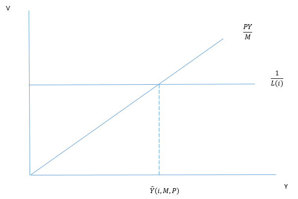
This gives us a level of output which is consistent with the demand for money for any given price level and nominal interest rate. This will be increasing in i (since L_i<0), decreasing in P and increasing in M. Call this function the “MV curve.”

RG/MV

At this point we have to deal with inflation expectations. One key feature of this model is that it is very explicit about which interest rates it is talking about where and so you have to deal with inflation expectations explicitly as well. This eliminates another one of my pet peeves about IS/LM (the more important one). The simplest way to do this is to assume that they are exogenous, and don’t depend on any of the other exogenous variables. Then, in equilibrium, the Fisher equation must hold.

i=r+π^e

Then we can rewrite the RG curve as RG(i-π^e). Then we have a nice downward-sloping RG curve and upward-sloping MV curve in i/Y space. Equilibrium in both the real goods market and the money market will determine a quantity of total output demanded and a nominal interest rate for any given price level. (Consumption, investment, velocity, and the real rate can all be easily recovered from this.)

Figure 3

Aggregate Demand

The aggregate demand curve is then a function giving all combinations of output and price which make up an equilibrium in both the real goods market and the money market. It can easily be seen that this is downward-sloping in price. If the price is higher, PY/M will shift to the left in figure 2 which will cause the MV curve to shift to the left and imply a lower aggregate quantity demanded. Furthermore, we can deduce how the curve will shift when the following exogenous variables change.

Money supply

If the money supply increases, this will shift PY/M to the right for any given P, which will cause the MV curve to also shift to the right and cause the aggregate quantity demanded for any given P to be higher. Note that for a given price level, and inflation expectation, this will lower the nominal rate, increase investment and decrease velocity. The degree to which the increase in money is absorbed by a decrease in velocity vs. an increase in aggregate quantity demanded depends on the slope of L(i).

Inflation expectations

If inflation expectations increase, this will cause RG(i-π^e) to shift to the right since any level of i will represent a lower level of r. This will cause the aggregate quantity demanded to be higher for any given P (an increase in aggregate demand). Note that this will cause an increase in i, but a decrease in r since the RG curve will shift up by exactly the amount of the increase in inflation expectations but it will move along the MV curve. This will mean an increase in output, investment and velocity.

Time preferences

If people become more impatient and want to consume more today, this will cause a decrease in investment supply and higher real rate for any given level of income which will cause the RG curve to shift to the right. This will cause the nominal rate, velocity and aggregate quantity demanded to increase for any given P.

Investment opportunities

If a new technology is discovered which increases the marginal product of investment, the demand for loanable goods will increase.  This will cause the RG curve to shift to the right and the AD curve to do the same, which will increase investment, output and real and nominal interest rates.  Note, that this may crowd out some consumption, depending on the shape of the indifference curves.

“Animal spirits”

If people decide they want to hold less money—L(i) decreases—then 1/L(i) will be higher for any given i which means that the MV curve will shift to the right and the nominal and real rates will be lower, aggregate quantity demanded, velocity, and investment will be higher.

Remarks

This model has two main benefits compared to IS/LM. One is that it has a bit more “micro foundations” in that it explicitly incorporates consumer preferences and demand for investment by firms. The other is that it carefully distinguishes between real rates and nominal rates which makes the transmission mechanism for monetary policy much more clear in my opinion. It also fits better with my framework of thinking about AD as Y=MV/P and dividing things into their effects on M and V rather than thinking in terms of C+I+G+NX and dividing things into their effects on those respectively (although note that you can still do that with this model).  I see this as a sort of monetarist version of IS/LM, though I don’t know if people with monetarist street cred would agree with me or not.

So far I haven’t explicitly tried to incorporate fiscal policy. To do this would require you to make some assumptions about how it affects peoples’ preferences and where the money comes from. (Is it from taxes or borrowing? If the latter, is it borrowed from the private market or from the central bank increasing the money supply?) Note however, that these questions are central to determining the effect of such policy.  You probably could just slap it onto AD if you wanted to assume that there were no effect on preferences (no crowding out) and you could change the household budget constraint to Y-T.  If the government borrows, you could add their demand to the demand for loanable goods.

Sorry the figures look like crap.  I need to figure out a better way to get them into wordpress

 

 

C+I+G+NX is a Stupid Way of Teaching Aggregate Demand

I took another step in my slow transformation into a macro guy this quarter by teaching introductory macroeconomics for the first time. I have taught intermediate once and a little bit of intro in a combined class at a school that was on semesters but frankly, I didn’t cover much macro in that one. So working through the introductory treatment of AS/AD was a little bit of a rough process and I suspect I learned the most out of everyone involved, which is not exactly ideal but has some redeeming value nonetheless.

This was only partly due to my lack of experience. It was also largely due to what I consider to be a severely flawed approach to teaching this stuff at an introductory level. I started out just following the textbook they gave me, but by the end I was sort of blazing my own trail. I am beginning to see what I think is a much better way of doing this. So I am writing this mostly for my own benefit, to help organize my thoughts for future classes. But I welcome feedback.

I have two main gripes with the standard treatment of AS/AD. The first is best illustrated by this question from my textbook.

Describe whether the following changes cause the aggregate demand curve to increase, decrease, or neither.

1. The price level increases.

2. Investment decreases.

3. Imports decrease and exports increase.

4. The price level decreases.

5. Consumption increases.

6. Government purchases decrease.

The reasoning behind this question is probably obvious. At the very beginning of the chapter they define aggregate demand as the following.

AD=C+I+G+NX

So obviously if investment increases, that must increase aggregate demand right? That makes sense if you implicitly assume that C, G and NX all stay constant. But that’s a silly thing to assume. Obviously, each of these things is endogenous. They must be or else there would be no P in that equation and then it wouldn’t make sense to call it aggregate demand. So they must mean:

C(P,….)+I(P,…..)+G+NX(P,…..)

So at the very least, I(P,…) is an exogenous demand for investment at different price levels.   So just saying “investment increases” is reasoning from a quantity change. What you mean by “investment increases” must be “demand for investment increases.” But then you haven’t said anything other than “assume that aggregate demand increases, what is the effect on aggregate demand?” In which case, you haven’t really explained anything. In order to say anything interesting about how aggregate demand changes, you have to say what would cause an increase in demand for investment. And the things that change the demand for investment, sometimes also effect something else in there, and not always in the same way.

For example, you might say that a decrease in interest rates causes investment demand (as a function of the price level) to increase. But now you are reasoning from a price change. Why did interest rates fall? Did people become more patient? If they did, then you have an increase in the supply of loanable funds, a fall in the interest rate, an increase in investment demand and a decrease in consumption demand. Does that increase or decrease aggregate demand? Hmmmm……

On the other hand, what if you have a decrease in expected inflation. Does this change real interest rates? If not, what happens to demand for consumption and investment? If so, why? And then how does it change demand for investment and consumption? What if the central bank is setting a lower nominal rate and this is increasing inflation expectations and also lowering the real interest rate in the short run? This probably means investment demand is increased and consumption demand is also increased since people will want to consume more and save less at the same time that firms want to invest more.  If this is the case, how is it that interest rates are lower again?

These are the difficult questions one has to grapple with in order to figure out macroeconomics. And to be sure, you can’t explain them all satisfactorily in an intro class. You have to make some assumptions that simplify things. But the problem with this C+I+G+NX approach is that it forces students to reason in a way that doesn’t really make sense without them realizing that it doesn’t make sense and it makes them less capable of grappling with these questions in the future instead of more capable because it trains them to think carelessly.  It’s an intellectual dead-end street.

We should be teaching them to think carefully, organizing information in the way that is the most helpful for understanding the essence of the problem and keeping careful track of what assumptions go into that formulation. Instead, it seems like introductory macro is designed to give them as much random information to memorize as possible to keep them from thinking carefully enough about what is going on to realize that it doesn’t really make sense.

For instance, in their quest for more material to memorize, they give three reasons that the AD curve is downward sloping: the wealth effect, the interest rate effect and the international trade effect. These all amount to “when prices are higher, people can’t afford to buy as much” except the first one is this notion applied to consumption, the second is the same concept with respect to investment and the third is sort of the same concept with respect to net exports (I want to avoid going off on a tangent about international trade so I am going to glance over most of the stuff related to that). So why not just call this the “wealth affect” and say that it applies to both consumption and investment?

Next, we come to my other main gripe. When they are talking about things that shift the AD curve, the first thing they mention is changes in real wealth. Here is how they describe changes in real wealth.

“One determinant of people’s spending habits is their current wealth. If your great-aunt died and left you $1 million, you’d probably start spending more right away: you’d eat out tonight, upgrade your wardrobe, and maybe even shop for some bigger-ticket items. This observation also applies to entire nations. When national wealth increases, aggregate demand increases. If wealth falls, aggregate demand declines.

For example, many people own stocks or mutual funds that are tied to the stock market. So when the stock market fluctuates, the wealth of a large portion of the population is affected. When overall stock values rise, wealth increases, which increases aggregate demand However, if the stock market falls significantly, then wealth declines and aggregate demand decreases. Widespread changes in real estate values also affect wealth. Consider that for many people a house represents a large portion of their wealth. When real estate values rise and fall, individual wealth follows, and this outcome affects aggregate demand.

Before moving on, note that in this section we are talking about changes in individuals’ real wealth not caused by changes in the price level. When we discussed the slope of the aggregate demand curve, we distinguished the wealth effect, which is caused by changes in the economy’s price level (P).”

So when prices go up, you get poorer and move along the AD curve. Unless it is prices of stocks or houses, then you get richer and the AD curve shifts to the right. If this seems confusing, then you are probably thinking too clearly.

According to the book, the great depression was caused (partly) by the stock market crash of 1929 and the “great recession” was caused (partly) by the housing collapse of 2008. These are both wrong. The causality goes the other way. Financial markets react to changes in expectations about the future rapidly, so systemic problems with the economy tend to show up first in the markets.

If you are talking about the prices of all real estate or all stocks falling, are you talking about a change in relative prices or a change in the price level? If you are talking about the former, then a) why is that happening? And b) isn’t someone else’s real wealth increasing because they don’t own real estate and now they can buy more of it? How is it that some changes in relative prices make us poorer on aggregate and some make us richer?  The book offers no clear explanation for this.  If it is not a change in relative prices but a change in the price level, then isn’t it a movement along the demand curve, not a shift?  And if that’s the case, does that mean the AD curve is upward sloping?

These are questions you might ask if you were trying to figure out this whole AD thing.  It’s not exactly that they all can’t be answered, but the C+I+G+NX framework doesn’t help you answer them.  It makes it more difficult to wrap you mind around.  If you are trying to actually get to the heart of this thing, this is what you actually need to ask and answer

Q: Supply and demand for apples are measured in other goods that people are willing to trade/accept for apples. What is the demand for all goods measured in?

A: Money. AD represents people’s willingness to trade money for goods (consumption, investment, whatever). This means that it is all about the willingness of people to hold money. It’s all about money.

Now, why is AD downward sloping and what shifts it? To see this, instead of starting with Y=C+I+G+NX, ignore that because it doesn’t tell you anything worthwhile about what aggregate demand means or how it works, and instead start with this:

MV=PY

The equation of exchange. Like the first equation, this is also an identity. It must be true. Unlike the other equation, it highlights what actually matters. For starters, it has Y and P in it, so a student can easily derive an AD curve from it for a given V and M and see why it must be downward sloping. In short, this is because of the “wealth effect” described in the textbook, but now you can clearly see that it is just one effect which applies to money. If prices are higher, for a given amount of money and a given velocity, people can’t afford to buy as much stuff. This applies to both consumption and investment (and net exports as long as you assume they have to be purchased with domestic currency). So the downward-sloping part is pretty straightforward (again, assuming, for now, that velocity is constant).

Why does it shift? Well we can see easily that (for a given V) if you increase M, it will shift to the right. You don’t have to try to explain that increasing M lowers the interest rate and lowering the interest rate increases investment and deal with all of the implicit assumptions that are hidden in there. All of those assumptions are replaced by the assumption “V is constant.”

Similarly, if you hold M constant, then anything that shifts the AD curve must do so by changing velocity. This is the type of fundamental insight which is completely absent from the C+I+G approach. So take the things that the book says shift AD:

Real wealth: as we have already established, this is dumb.

Expected future prices: If people expect future prices to be higher, they will want to hold less money, they will want to buy more stuff today, velocity will increase and AD will shift to the right.

Expected future income: It’s actually not entirely clear that this should increase AD but here is what must happen if it does. Either it must make people want to hold less money at a given price level (and increase velocity) or it might increase the money supply. If banks are not reserve constrained, then people may borrow more and increase the broader measure of the money supply (or if you prefer, increase the velocity of M0).  Or if the central bank is targeting an interest rate, it might increase the money base as demand (supply) for loanable funds increases (decreases).

Furthermore, you can take government spending.  Instead of just saying “well it increases G so that’s an increase in AD right there” which is dumb.  You have to ask yourself difficult but interesting questions.  For instance, where does the money come from?  Maybe you increase taxes.  In which case shouldn’t that just crowd out private consumption? Yeah probably but how much does it decrease consumption?  Well you can go through the whole spending multiplier thing and argue (notice I’m not saying “show”) that when the government takes your money and spends it, it causes more total spending than if they just let you spend it.  Why?  Because you will hold less money that way, or in other words, it will increase velocity.

Alternatively, they could borrow it.  Who do they borrow it from?  If they borrow it from the private economy then won’t this crowd out private investment?  Yes.  To what extent?  Well, try to make some kind of argument that it will increase or decrease or not change velocity.  What if they borrow it from the central bank?  Then it’s an increase in M (and it’s really monetary policy) and it’s very clear how this will affect AD.

You wanna talk about “animal spirits?”  That’s basically just a way of saying that velocity drops for some reason we don’t understand and can’t explain.

Now of course, it is equally true that V probably won’t remain constant when the money supply changes, but now you have focused attention clearly on the important thing. Remember AD is all about peoples’ willingness to hold money.  And this is also the essence of Velocity. So we can start with the quantity theory (constant velocity) of money and then start asking what would cause velocity to change. And if you want, you can make velocity a function of the price level.

Let’s say that you think that velocity will be lower if prices are higher because when the price level is higher, it will take more dollars to equal the same amount of real money balances. You can explain that the AD curve will still be downward-sloping as long as the price elasticity of velocity is inelastic. At this point your intro class will probably look at you with glazed-over eyes but the point is that everything about AD depends on the quantity of money and velocity. All of the things that textbooks talk about shifting the curve by increasing investment or something like that are either wrong or they affect velocity. Instead of teaching them to think about C+I+G+NX, we should teach them to think about PY=MV. You can make velocity a function of whatever you want. But then you are concentrating on what matters. The fundamental forces which drive aggregate demand.

C, I, G, and NX are not the fundamental forces driving aggregate demand, they are just categories that you can divide it into. The fundamental force driving aggregate demand is the willingness to spend money on goods. It doesn’t matter if those goods are consumption or investment. The only thing that matters is how much money there is and how willing people are to hold that money instead of spending it on something. If you can grasp this concept, you get aggregate demand. If not, you don’t. If something affects AD, it must affect one or both of these. If you can see how it does that, you get it. If not, you are probably confused.

Now, this is all consistent with the model of aggregate demand taught in introductory macro, it’s just a better way of teaching it, in my opinion. When you get to intermediate, I have a similar set of gripes. So I am coming up with a better way of doing IS/LM. Coming soon.

Land Theory of Value

Nick Rowe has (tongue-in-cheek) post about the land theory of value.  I know he isn’t pushing that theory but as an exercise, let me try to address his ultimate question:

Plus, the Land Theory of Value is worth considering in its own right, or simply as an exercise in studying value theory. Why is it wrong? What are we looking for in a theory of value? What counts as success?

Bound up in this question is the question “what is value anyway?”  I think what most classical, and modern mainstream economists are looking for in a theory of value is a way to explain (relative) prices.  In other words, when they say “theory of value” they mean “theory of relative prices.”  They take for granted that prices are a measurement of “value” and try to construct a theory that explains how this is true.  This seems to be what Nick is after.

On the other hand, in my opinion–and internet Marxists will probably argue with this– the Marxist version of the labor theory of value is an attempt to define “value” independently of prices and then construct a theory which says that market prices are not representative of “value.”  If this is the case, then you have a way of claiming that mutually voluntary (or, in other words, free) trade can be exploitative (someone wins and someone loses) and this is a foundational assumption underlying most Marxist rhetoric.

So if you take the latter approach and assume that all value comes from labor, then nobody can prove you wrong.  If they say “okay, but what about this diamond, it is highly valuable but it takes very little labor to produce it,” you just respond “no, it isn’t highly valuable, because it didn’t take very much labor to produce it.”  And if that makes you uneasy, then maybe you make up alternate definitions of value like “use value” and “exchange value” so that you can avoid reconciling your definition of value with the actual prices of things.

So I think most economists find the latter approach unappealing.  The standard (subjective) theory of value also defines value independently of prices.  Value means the quantity of other goods (somehow measured) which someone is willing to give up for something.  This value is subjective and there is no attempt to explain where it comes from.  We merely assume that people have some willingness to trade goods for other goods.  A nice feature of this definition of value though is that, once you use it to explain prices, you find that prices are, in fact, a measure of value (specifically marginal value).  So if, when you say “a theory of value,” you really mean “a theory of prices,” then this theory works for you, because it does explain prices.

Now what Nick seems to be describing is a theory of prices.  He (or technically, his Dutch ancestor) is basically arguing that you can explain the prices of things in reference to land.  It is not an independent theory of “value” (meaning independent of prices).  It takes for granted that price is a measure of “value” and seeks to explain these measurements.  But the theory described here does not explain these at all, it only shows that prices can be measured by a standard unit of land.  This should not be surprising if you believe in the standard (subjective value) theory.  In that model, you can measure the value of any good in terms of any other good.

Take this part.

You have to consider the marginal land, that is exactly on the margin between producing wheat and producing barley. If that marginal land could produce two tons of wheat or four tons of barley per acre, then the value of one ton of barley must be half the value of one ton of wheat. That way we can compare the value of land that only grows wheat to land that only grows barley. And the market prices will themselves tell us the relative values of all different sorts of land, so we can convert them all to standard land.

So you can observe the marginal rate of transformation between wheat and barley and that will be equal to the price.  That’s fine.  But that does nothing to determine why the margin is where it is.  If there is a concave PPF, then the marginal rate of transformation between wheat and barley depends on how much of each the society chooses to produce.  How do they determine how much wheat and how much barley to produce?  Well if you believe in subjective value, then they buy whatever they value more until, on the margin, they are indifferent between $1 worth of wheat and $1 worth of barley (or if you prefer, you can measure the market price in any other good).  This subjective value, along with the various production possibilities, determines a price.

If you wanted to, you could take some wheat land and use it to raise cockroaches.  Assuming that no land is being used for this and the market price of cockroaches is negative (you pay to get rid of them).  Do we conclude that the true “value” of cockroaches is determined by the amount of cockroaches you could raise on a “standard” unit of land?  If so, is the price wrong?  The lack of an existing margin also presents other problems but it’s not necessary to go into them.  The point is that chickens are more valuable than cockroaches not because they take more land to produce but because we subjectively are willing to give up other goods for one and not the other.

Now, of course, if things work the way the standard theory says, then the relative price of wheat and barley will be equal to the marginal rate of transformation between the two.  So if you can observe the marginal rate of transformation, you can observe the price.  But this is different from explaining the price.  In order to do that, you have to explain why the margin is where it is.  And in order to do that, you need subjective value.  Of course, Nick pointed this out to his ancestor and his ancestor made a meaningless reply.

Preferences! We cannot observe preferences. Land is real and objective. And the margin of cultivation between wheat and barley is real and objective, and we can observe it. We don’t need no stinking preferences to determine value!

But, again, the only difference between preferences and the margin of cultivation is that the latter is observable and the former isn’t.  So if all you want in your theory is a way of observing value, then this works fine.  But if you want to explain value, then you need subjective preferences.  And besides, if you just want to observe value, you can just look at prices.  So what is the point of a supposedly deeper “theory” based on land which only amounts to a more difficult way of observing the same thing?

The same argument applies to Van Rowe’s argument about crop rotation.

If there are three different crops, and three different ways of rotating them that are not linearly dependent, and all three rotations produce the same rate of profit, as they must, it is trivial matrix algebra to solve for the values of each crop.

There is no sense, independent of market prices, in which all 3 rotations must have the same profit.  They must have the same profit only if prices are such that the farmer is indifferent between them.  In a large market like those that people like me imagine, this will always be the case somewhere for someone and therefore, in theory, if you could find all of the marginal farmers and observe their production matrixes, you could back out the market prices.  But, again, you would not have explained why those margins are where they are.  In order to do that, you need a market to determine prices and that requires a demand curve, and that requires preferences.

All of this is ultimately equivalent to saying: “Supply determines the price, you don’t need demand.  See, we can always just look at the marginal cost of production and figure out the price.”  That’s nonsense, and so is this theory.

 

 

Et Tu, Nick Rowe?

Nick Rowe has another post about “red money.” I love these posts because they are very close to the concept that I am trying to advance regarding the relationship between money (which Nick sometimes calls “green money”) and debt (which he sometimes calls “red money.”) But I have two gripes with this one. One is his abuse of the concept of utility, which some people who have read me before may roll their eyes at, but since I have assumed the role of internet utility policeman, I can’t let it slide. However, I will save it for last. The other is his insistence that his red money is not a debt.

Now, what is this a theory of? It’s not simply debt, because debt is an asset of someone. Red money is an asset of no one.

This is purely semantic of course, but I kind of take it as a shot at folks like me who like to talk about debt, so I feel compelled to point out the fact that it is purely semantic and based entirely on an entirely unrealistic assumption of his.

This conclusion is based on the notion that the red money is not an asset of anyone. But red money is an obligation to pay real goods in the future to someone. It’s just that the obligation is to a group of people (future young people) rather than to a specific individual. Therefore, it is difficult to say that any particular individual holds an asset.

However, in order to make this work, he has to make the (unrealistic) assumption that people have to dispose of all of their red money before they die. In reality, if you had red money, in the sense it is described, people would just accumulate vast amounts of red money and then never pay it back (sell it back?). The reason for this is precisely the reason that Nick claims it is not a debt, namely that no particular person holds an “asset” on the other end of that debt which could require them to pay.

Nick, of course, is aware of this and he deals with it by assuming that there is some punishment in the afterlife for dying with red money. But this assumption only serves to take the asset out of this mortal coil and place it instead in another realm. So, if you want, you can imagine that God holds the asset on the other end of your liability and it will be him that extracts payment if you fail to transfer it to someone else before death, but that is not changing the fundamental nature of the debt.

Of course, in real life, this wouldn’t work because many people would not believe that God would punish them if they didn’t sell all of their red money. So if you wanted to actually make red money work in a way similar to what Nick describes, you would need to come up with some way to punish people on earth for accumulating too much red money.

One way of doing this would be to create some kind of entity, on earth, that would hold the asset on the other end of the liability which is red money. This entity could then take the goods from the old and transfer them to the young, along with the requisite amount of red money. Then you would have a specific contract with that entity which would require you to pay real goods in a given timeframe and if you didn’t, that entity could come after you for the goods. At this point, someone would hold an “asset” for each unit of red money, and I think it would be difficult to argue that it was not a debt.

Of course, if that entity didn’t want to deal with collecting and distributing real goods, they could also issue another kind of notes, let’s call them “green money” to the young, along with their red money, and they could allow the old to use this green money to cancel out their red money. Then the young would trade the green money for goods from the old and the old would use the green money to repay their debt to the entity which issues red and green money and keeps track of who owes what (which is another way of saying that they hold the assets backing the red-money debts). Then they wouldn’t have to bother with real goods except in the event that some old person failed to come up with the requisite quantity of green money in the allotted time period.

Now I have no problem with making unrealistic assumptions in order to make a point, but if the point you make is driven entirely by an unrealistic assumption and when you replace it with a more realistic assumption that point is no longer valid, then you have a bad assumption (or a bad point depending on how you want to look at it).

So whose model seems more realistic, Nicks, in which red money is “not a debt” but people always resell it out of fear of punishment in the afterlife, or mine, in which red money is a debt and people resell it out of fear of having their stuff taken by the issuer of that debt? If it’s mine, then maybe we should think about the role that debt plays in all of this and not dismiss it as an unimportant detail.

Now, regarding utility, it is becoming apparent to me that it is macro people who are driving this particular regression in economic understanding. And the reason is somewhat understandable. Put simply, it’s easier to just assume diminishing marginal utility in each period than to assume the correct thing which is that people have diminishing marginal rates of substitution between consumption in each period. If Nick had proposed the same model, with the same equations and said that, I would have no beef.

Notice that his utility function, also exhibits the latter property, and it is that property which drives the results, not diminishing marginal utility. To see this, you can simply plug in a utility function which has increasing marginal utility and also diminishing MRS (for instance (cy^2)(co^2)). So Nick probably thinks it doesn’t matter whether you say it his way or my way, and I would have rolled my eyes and held my tongue if he hadn’t gone on to say this [emphasis added]:

“Diminishing Marginal Utility. If U=log(C), then dU/dC=1/C, which is a decreasing function of C. Every extra apple you eat per day gives you less and less extra utility. So you would rather eat 10 apples every day, than 9 apples on even days and 11 apples on odd days. And 0 apples on even days and 20 apples on odd days, would be even worse. We want to smooth our consumption across time periods (and across states of the world, because insurance is motivated by the same thing).”

So it’s not just a convenient mathematical assumption he is making, he is justifying that assumption with a defunct philosophy, with no theoretical or empirical justification, which the profession discarded a century ago. (Please note that I am talking about DMU not consumption smoothing, which I have no problem with, but which can be generated by diminishing MRS without resulting to making conjectures about purely hypothetical things like “satisfaction” or “happiness.”)

This corrupts peoples’ understanding of a concept that is at the heart of much of economics and it is frustrating to those of us who have to try to teach people intermediate micro in the proper way (at least those of us who care about getting this right which, much to my consternation,  seems to be a dying breed, …..). I wish smart, reputable, economists, whom I know are capable of comprehending the distinction, could refrain from falling back on this type of logic.

So I’m writing Nick a citation from the internet utility police department. If he fails to correct the violation, there will be no consequences, since it’s a department I made up and I have no real power or sway with anyone. Except, of course, that a bunch of people may read your stuff and become confused about what utility means, or heaven forbid, become utilitarians. May their intellectual blood be on your hands. (Maybe there will be some penalty in the afterlife…)

 

P.S. Just for the record, I’m being smug here, I love Nick Rowe and I hope his afterlife is filled with nothing but happiness and satisfaction. But if it is, I hope he doesn’t describe it as a high level of utility.